3.11 Degree of Financial Leverage and Degree of Total Leverage

In this section we explored operating leverage which is sometimes referred to as first stage leverage and in the early topic on the DuPont decomposition we introduced the term financial leverage.  The degree of financial leverage results from a second stage analysis of Earnings Before Taxes (EBT) and Earnings Before Interest and Taxes (EBIT). 

Alternatively, when viewed from the perspective of the Income Statement we can define the degree of Financial Leverage in terms of Net Income as follows:

Degree of Total Leverage

This number relates a firm’s operating and financial leverage to its net income.  This is a useful number for financial analysts to assess because it allows earnings’ forecasts to be made starting from Sales.  However, first we consider the operational details including how to estimate this number from the financial statements.  In relation to Sales Revenue the Degree of Total Leverage is defined as follows:

That is, by starting with the problem of forecasting sales revenue then the Degree of Total Leverage can relate this forecast to an earnings’ forecast.

We can further decompose the Degree of Total Leverage into the product of its two drivers, the Degree of Operating Leverage times the Degree of Financial Leverage.  In this form it can be related directly to the Contribution Margin format of a Variable or Direct Income Statement as follows:

Next consider how this is computed from the financial statements.

Tutor Reconciliation:  Proctor and Gamble (PG)

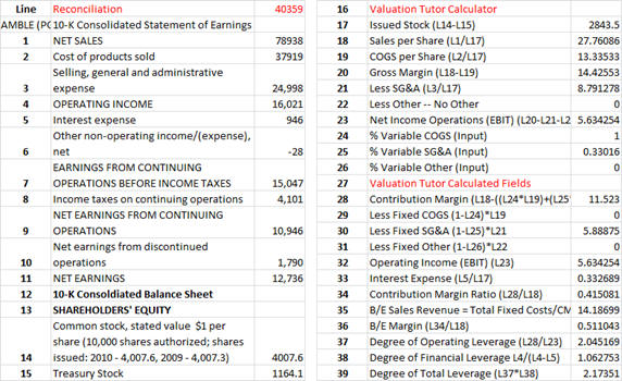
Our objective is to reconcile the following from the 10-K:

Step 1:  Now bring up two Income Statements for Proctor and Gamble as described in section 3.2 as displayed below. 

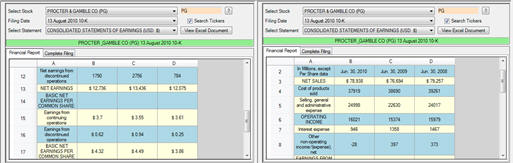
For Proctor and Gamble you can see that the Cost of products sold = $37,919 and the “Selling, general and administration” expense =$24,998.  Plus now Interest Expense is $946.

To recast the income statement from its full or absorption costing format to a direct or variable costing format we need to break up these costs into their fixed and variable components.  For reconciliation purposes suppose we assume that 80% of the COGS are variable and 20% of the SA&G expenses are variable.  These percentages can be subject to more refined analysis later but for now we are more concerned with mastering the operational details.

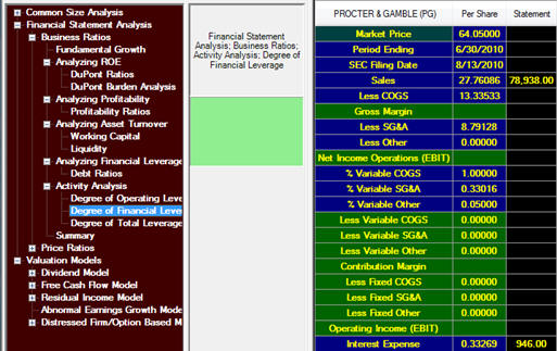
Step 2:  Click on Calculate and we can verify the input and derived fields for the following:

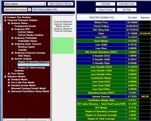
The above demonstrates the power of recasting the income statement in this manner.  This lets you estimate the Degree of Financial Leverage as well as the Break Even points for Sales Revenue and implied Margin of Safety (i.e., Sales minus B/E Sales.  The Degree of Total Leverage is the product of the Degree of Operating Leverage and the Degree of Financial leverage.

The reconciliation from the Income Statement is provided below.