3.10 Degree of Operating Leverage and Capacity
Degree of Operating Leverage
A firm’s operating leverage is defined as the percentage change in the firm’s operating earnings (EBIT less any non-operating income), that accompanies a percentage change in the contribution margin. That is, the operating income elasticity with respect to the contribution margin. This important number predicts for an analyst what the percentage change in operating earnings is given the percentage change in sales revenue. As a result, this number is important for predicting EBIT given the predicted growth in Sales Revenue. The consensus sales revenue forecast is readily available and the DOL provides an EBIT forecast given this consensus number.
Formally, the definition of DOL is:
Degree of Operating
Leverage (DOL) = % Change in operating income / % Change in
sales revenue
Equivalently,
Degree of Operating
Leverage (DOL) = Contribution margin / EBIT
This important measure
reflects the fact that a change in Sales can lead to a more than
proportional change in earnings from operations.
In particular, the higher the degree of operating
leverage the higher the predicted change.
However, the relative size of the Degree of Operating
Leverage is affected by how close the firm is to their
break-even point.
The closer the higher is the DOL.
The above equivalence relationship is not immediately obvious. Understanding this requires reviewing the basics of cost volume profit (CVP) analysis first and then we will derive the above equivalence relationship.
Cost Volume Profit Analysis
Cost volume profit analysis studies the relationship among sales, variable costs and fixed costs. It assumes that linear costs provides a good description of real world cost behavior. From this assumption the accounting income statement can be restated in avariable costing format as follows starting from the traditional gross margin or absorption format::
Absorption Costing:
Sales
Less COGS
Gross Margin
Less Marketing and
Administration
Net Income from
Operations (EBIT)
A variable cost income
statement highlights cost behavior (i.e., variable versus fixed
costs) and contribution margin.
This immediately ties in to a cost/volume/profit break
even type of analysis:
Variable Costing
Sales
Less Variable COGS
Less Variable
Marketing and Administration
Contribution Margin
Less Fixed Overhead
Less Fixed
Marketing and Administration
Net Income from
Operations (EBIT)
The above format allows an analyst to immediately estimate the following important concepts:
Contribution Margin (CM) = (Sales Revenue – Total Variable Costs)
Contribution Margin
Ratio (CMR) = (Sales Revenue – Total Variable Costs)/Sales Revenue
Sales Revenue*Contribution Margin Ratio = Contribution Margin
The usual immediate relationships to derive from cost volume profit analysis is to compute break even sales revenue and break even margins as follows:
Break Even (B/E)
Analysis ($Sales Revenue)
= Total Fixed Costs/(Contribution Margin Ratio)
Break Even (B/E)
Margin = B/E $Sales Revenue/$Sales Revenue
However, we are currently interested in deriving the equivalence relationship from the definition of DOL and the concept of contribution margin.
Derivation of Equivalence Relationship for Degree of Operating Leverage (DOL)
At the beginning of this topic we defined DOL and the equivalence relationship can be derived as follows:
Degree of Operating Leverage (DOL) = % Change in operating income/%
Change in sales revenue
Assuming fixed costs remain unchanged and EBIT = Sales - Variable
Costs - Fixed Costs, it follows:
%ΔEBIT = Δ(Sales - Variable Costs))/EBIT = ΔCM / EBIT
%ΔSales = ΔSales / Sales
Taking the ratio of the above two equations and re-arranging:
%ΔEBIT /%ΔSales = Sales(ΔCM/ΔSales) / EBIT = Sales*CMR / EBIT = CM
/ EBIT
That is:
Degree of Operating Leverage (DOL) = Contribution margin / EBIT
In the next example we apply these relationships to the 10-K data:
Tutor Reconciliation:
Proctor and Gamble (PG)
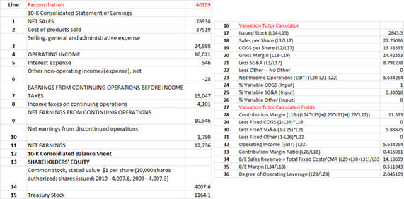
Our objective is to reconcile the following from the 10-K:
Step 1:
Now bring up two Income Statements for Proctor and Gamble
as described in section 3.2 as displayed below.
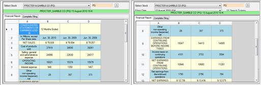
For Proctor and Gamble you can see that the Cost of products
sold = $37,919 and the “Selling, general and administration”
expense =$24,998.
To recast the income statement from its full or absorption
costing format to a direct or variable costing format we need to
break up these costs into their fixed and variable components.
For reconciliation purposes suppose we assume that 80% of
the COGS are variable and 20% of the SA&G expenses are variable.
These percentages can be subject to more refined analysis
later but for now we are more concerned with mastering the
operational details.
Step 2:
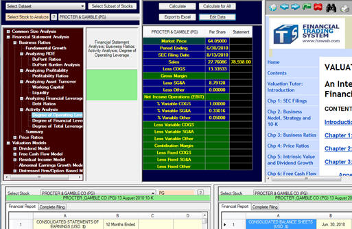
Click on Calculate and we can verify the input and
derived fields for the following:
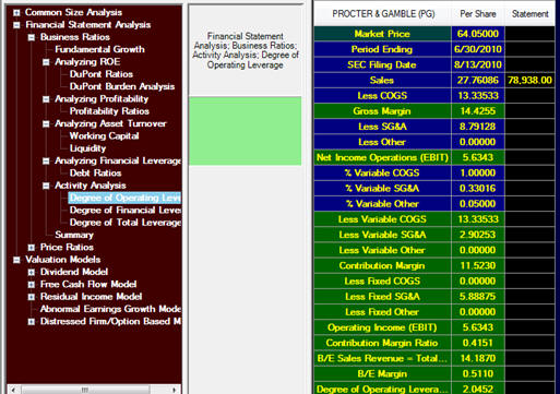
The above demonstrates the power of recasting the income
statement in this manner.
This lets you estimate the Degree of Operating Leverage
but in addition it further lets you estimate Break Even points
for Sales Revenue and implied Margin of Safety (i.e., Sales
minus B/E Sales.
Cost Behavior Assessment Remark:
Observe above that the % Variable COGS, % Variable SG&A
and % Variable Other are numbers inputted into the calculator.
Where do these numbers come from? There are various approaches
used by professionals in the field for assessing these numbers.
Clearly, managers’ inside a firm have access to better
information than financial analysts outside of the firm.
However, financial analysts can still make reasonable
assessments of the cost behavior.
Interested readers are encouraged to work through
questions 7-13 in the problem set at the end of this chapter.
In particular, Question 9 provides the details for
estimating cost behavior using regression analysis.
Reconciling from the Income Statement
The reconciliation from the Income Statement is provided below.
: