
6.12
The 2 Stage Model
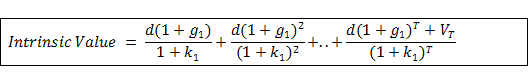
The intrinsic value in the two stage
dividend model is calculated as follows:
In the
two stage model, dividends grow at rage g1 for T years
and then grow at rate g2.
The dividends are discounted at rate k1 in stage 1
and at rate k2 thereafter.
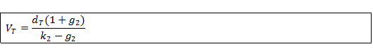
This yields the following formula for the intrinsic value:
Where
Abnormal Growth:
Also known as “extraordinary growth,” this is the growth
projected over the next finite number of years (typically 5-years-
10-years). As an
aside, when you are calculating the intrinsic value for a firm that
has negative short run growth, you want to use a three stage model,
where the first two stages provide a further breakdown of the growth
rates into three phases --- a first phase of negative growth,
followed by a second phase of abnormal positive growth and then
ultimately a third phase of normal growth.
Normal Growth:
Ultimately in every multi-stage growth model of intrinsic
value you must make some simplifying assumption that in the final
stage the (going concern) firm grows in perpetuity at some normal or
stable growth rate. To
avoid the limiting case implications discussed in relation to the
Constant Growth we assume that Normal Growth is bound from above by
the economy wide growth.
Therefore, to estimate Normal Growth we start with reviewing the
behavior of long run economy wide growth behavior.
Estimating Normal (Stage 2) Growth
Normal growth in a 2-stage model is bound
by the economy wide growth.
This number can be estimated by referring to long term
average macroeconomic data for
the US economy. In Valuation
Tutor’s information system, under “Papers and Reports,” you will see
a link to a report on the long term growth rate of the US economy:

The following
quote comes from this report:
We also observe over the last
100-year span that the rates of economic growth across the then
emerging industrial nations were fairly tightly clustered around
this 2.0% pace. At the high end was Japan with an annual rate of
growth averaging about 2.7%, while at the low end was Great Britain
with an annual growth rate averaging 1.4%. The United States, which
grew at a 1.8% average annual rate, was slightly below average.
They also went
on to observe:
For the United States, the long-term
growth of real GDP per capita over the last 125 years has revealed
remarkable steadiness, advancing decade after decade with only
modest and temporary variation from the observed 1.8% annual rate of
increase.
The estimates in
these quotes are for the growth of real GDP, which does not take
into account inflation.
In valuation exercises, we require the growth rate of nominal GDP,
which takes into account inflation (otherwise, we would have to
recast everything in terms of constant dollars!). Inflation numbers
suggest that inflation compounded from 1913 to 2008 resulted in a
cumulative rate of 2071.23%.
This implies an annual constant compounded rate of
approximately 3.24%.
Combining the
above we can make a reasonable estimate for one plus the long term
nominal growth in the US, to be around 1.018*1.03 = 1.04854.
In our examples,
we will use 4.5% as the stage 2 growth rate, slightly below the
economy wide rate. For a
company like IBM that has a strong track record on research and
development as well as filed patents, it makes sense to think it
mirror the long term growth rate of the economy.
The Length of Stage 1
The length of
stage 1 will depend on two sets of factors.
The first set is firm specific.
For example, a firm may have developed a successful new
product, and may enjoy a period of high growth before its
competitors can slow its growth. Patents would give a company an
advantage as well; for example, for a pharmaceuticals company, until
a patent expires, the company can enjoy high growth.
The second set
of factors concern the economy as a whole.
Growth will be affected by general economic conditions, such
as a prolonged boom or a prolonged slump.
The National Bureau of Economic Research dates the start and
end of a business cycle.
A business cycle measures fluctuations of economic growth around the
long term growth rate.
Generally,
analysts are unwilling to use large numbers for stage 1 because it
implies that current abnormal conditions are going to prevail for a
long time. Even if a
firm is experiencing rapid growth, competition will limit the
growth, so the time to market of competitors will limit the time.
One of the longest is patent protection to drug makers, which
is twenty years. But
even in that case, it is unlikely that sales or earnings will grow
at a rapid pace for the entire period.
And with economics fluctuations, the actual growth over the
period may be tempered further.
If you search
for examples of applications of the dividend model by analysts, you
find that they typically use 5 or ten years as the length of stage
1. Of course, if the
company you are studying has specific characteristics that inform
you about its growth period, you should certainly use that.