
6.11
Tutor Break: One Stage Dividend Model
Let’s
apply our estimates to IBM.
The current annual dividend for IBM is 2.191.
What should we use as the growth rate?
Currently, analyst forecasts for IBM’s earnings growth are
5.53%. If we use this
number, we get:
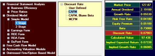
Besides the
calculated value, Valuation Tutor provides two other calculations:
the “implied expected return” and the “implied growth rate.”
The implied expected return is the ke that would
make the intrinsic value equal to the market price.
The implied growth rate is the growth rate that would make
the intrinsic value equal to the market price.
In this example, you can think of it as saying either that
the “market is pricing IBM as if it has a cost of capital or
discount rate of 7.338%” or as saying that the “market is pricing
IBM as if it had a growth rate of 6.085%.”
This inference is very important in making judgments about
the value of the stock; if the implied growth rate is too high to be
plausible, then you may feel that the market price is too high
relative to the intrinsic value.
Let’s go back
to the historical growth rate of dividends we calculated earlier.
We had found that over the last 50 years, IBM’s dividend has
grown by about 8%. What
if we use g=8%?
The model would
not work so well. The
growth rate would be greater than ke, and so the value
would actually be infinite.
Valuation Tutor would actually report a negative value; it
calculates d1/(ke-g) and if ke < g
while d1>0, the answer is negative.
You could argue
that the discount rate is too low, perhaps because we are using the
low end of consensus estimates for the equity premium. If we used
5.7% and the 7% growth estimate, we would get:
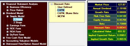
This is much
higher than the market price.
However, let us work a little longer with CAPM.
One observation about beta’s is that over time, betas tend to
drift towards 1. So if
a beta is low, it tends to become high, if a beta is greater than 1,
it tends to adjust downwards
The Blume adjustment accounts for this; it replaces beta by
Blume Beta = Beta *0.67 + 0.33 = 0.8191
If we use this in the IBM example, we get
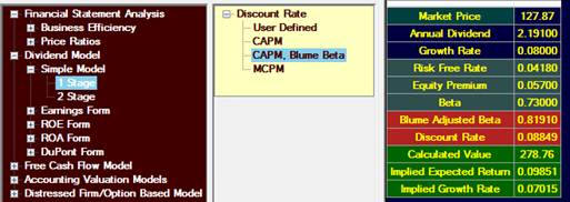
This obviously brings down the intrinsic value, and also gives you
some insight into how sensitive the model is to the inputs.
Finally, we mention some other consistency checks you can perform.
For example, since stockholders only get paid after
bondholders, IBM’s stock must be riskier than IBM’s bonds.
Therefore, ke for IBM must be at least as great as
the yield on IBM’s bonds.
This yield depends on IBM’s debt rating, and you can
typically find information about the rating in their 10-K (Part 2,
Item 7):
The major rating agencies’ ratings on the company’s debt securities
at December 31, 2009 appear in the table below and remain unchanged
from December 31, 2008. The company’s debt securities do not contain
any acceleration clauses which could change the scheduled maturities
of the obligation. In addition, the company does not have “ratings
trigger” provisions in its debt covenants or documentation, which
would allow the holders to declare an event of default and seek to
accelerate payments thereunder in the event of a change in credit
rating. The company’s contractual agreements governing derivative
instruments contain standard market clauses which can trigger the
termination of the agreement if the company’s credit rating were to
fall below investment grade. At December 31, 2009, the fair value of
those instruments that were in a liability position was $1,555
million, before any applicable netting, and this position is subject
to fluctuations in fair value period to period based on the level of
the company’s outstanding instruments and market conditions. The
company has no other contractual arrangements that, in the event of
a change in credit rating, would result in a material adverse effect
on its financial position or liquidity.
In addition, they provide the following table:

If the information is not available in the 10-K, you can look up the
current rating of the debt using the Bonds link in the information
system::
On the resulting screen, enter the ticker (say IBM) and you will see
a list of bonds issues by the company, their yields, as well as
their Fitch ratings.
If bonds are not listed, you can simply enter the ticker and
“credit rating” into your search engine; when we did this for IBM,
we found various reports that it had been upgraded to A+.
What is the yield on an A+ rated corporate bond?
Various bond rating sites give you this information; a free
source is the US Federal Reserve Board, which each provides Moody’s
seasoned rates for both Aaa and Baa bonds of a 10 year maturity.
At the time of this example these were:
Aaa = 4.89%
Baa = 6.28%
You can linearly interpolate to get:
Aaa = 4.89%
Aa = 5.35%
A = 5.82%
Baa = 6.28%
We will need to add a small “spread” to this to adjust for the fact
that we are using a 30-year Treasury yield (since we are discounting
over the long term). If
we add 1% (the Treasury 30 year yield at this time is 0.92%, or 92
basis points, above the 10-year treasury yield), we get 5.82 + 1.00
= 6.82%. This would be a
lower bound for ke.
An upper bound is 9.28% = 4.18% + 5.1%, which is CAPM applied
to a firm with beta equal to 1 and since IBM’s beta is less than 1.
This gives you a reasonable range for the ke.
At the lower rate, with a growth estimate of 5.53%, the value
comes out to 179.24; at the high discount rate, it comes out to
61.65. You can see the
interplay between the growth rate and the discount rate; if we use
the 8% growth rate and the high discount rate, the calculated value
is 184. If you think the
growth rate is somewhere between the analysts forecast of 5.53% and
the historical growth rate of 8%, then you can see that market price
is consistent with a discount rate somewhat higher than the CAPM.
Criticism of the One Stage
Model
The one-stage
model is obviously quite simple. For example, it assumes that IBM’s
dividend grows forever at a constant rate.
In reality we observe that
firms go through a life cycle, and so the growth rate over the near
term may be quite different from the long run growth rate.
This idea is captured by the two stage growth model, which
was also first analyzed by Williams in 1938.
The idea can be extended to multi-stage models, e.g. a three
stage model.