Binomial Tree Module

Introduction

This module introduces you to the option pricing problem in a simple binomial world.  In this world the price of the underlying can go up or down each period.  The two main advantages of this simplification are:

First, it lets you quickly become acquainted with the economic intuition that underlies the Black Scholes option pricing model.

Second, the binomial tree has resulted in numerical solutions to more general option pricing problems than what is covered by the Black Scholes model.  For example, the American put option can be valued this way.   

Applying the Binomial Tree Module

In the following example, we show that you can use the one-period binomial model to value an option.  The technique illustrated is the same as applied in the original Black Scholes option pricing paper.  This technique identifies the arbitrage free price of an option by creating a riskless portfolio synthetically, using the stock and an option.  Here, riskless means that the portfolio has a known value at the end of the period, no matter what happens to the stock price.  If the portfolio is riskless, then we know its current value.  This is simply the future value discounted by the risk-free interest rate.  Then, since we know the portfolio value and the stock price, we can immediately identify the arbitrage free option price from the difference.

From this approach we can interpret the arbitrage free option price in terms of the general principle of valuation.  This principle asserts that the value of any asset is the present discounted value of all future cash flows from the asset.  To value an option by applying this principle requires that we need to determine two things: the future cash flows and the discount rate. 

For a European option, the future cash flows are easy; for example, for a call option, the cash flow is 0 if the future stock price is less than the strike price, and equals the future stock price minus the strike price otherwise.

What about the discount rate?  

Here lies the problem.  We cannot use the risk-free interest rate, since the future cash flows are not risk-free; they depend on the unknown future stock price. If people are risk-averse, then they will hold risky securities only if they can get a return greater than the risk-free interest rate.  In fact, much of the problem in valuing risky securities is determining the appropriate discount rate, as in the capital asset pricing model. The fundamental riskless hedge argument solves the problem of determining the discount rate, since we can apply the risk free rate to discount the cash flows from a riskless portfolio.  

In example 1 below we first illustrate the principles underlying the riskless hedged portfolio approach to option valuation.  In the subsequent examples, we apply the FTS Binomial Tree Module to solve a set of specific option pricing and related problems.

Example 1:  Creating a Riskless Portfolio

Let S denote the current stock price and assume that at the end of one period the stock value is either 10 or 40.

In the display window set Asset Price to equal 20, strike price equal to 20, uptick to 2 and downtick to 0.5.   From the top drop down above the button Draw Tree select Asset Process, the second drop down select European Option and then click on Draw Tree.

We will first study the European put and call options with a strike price, X, of 20 when the risk-free interest rate is zero.

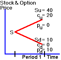
The future values of the stock and the options are depicted in the "tree" in Figure 2.1, which you can see by changing Asset Process to Put and Call option from the first drop down.  You can see that the tree values are the same as in Figure 2.1.

Figure 2.1

One-Period Binomial Tree

where, given an uptick, u, Su is the realized stock price, Cu is the realized call option value, and Pu   is the realized put option value.  You know, for instance, that Pu  is zero since the put option is worthless when S = 40 > X = 20.

Now suppose you form a portfolio:

Buy 2 stocks;

Sell 3 call options

Consider what happens at the end of the period if a downtick occurs.  Since the stock is worth 10, the call option finishes out-of-the-money and the trader you sold the call option to would not exercise it.  The final payoff from your portfolio is 20, which is the value of the two stocks.

Suppose an uptick occurs.  Each stock is worth 40, but the calls would now be exercised against you.  You would be required to give three stocks to the person who bought the options, and you would receive 20 for each stock.  Therefore, your final position would be:

+ 80 from the stock you hold;

+ 60 from the three options being exercised;

- 120 to buy the three stocks to give to the option exerciser;

which leaves you with 20.

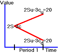
Therefore, no matter what the state (or final value  of  the  stock), you will end up with 20 at the end of the period as indicated in Figure 2.2.

Figure 2.2

A Riskless Portfolio

You now have a riskless portfolio.  The present value of this portfolio is 20 since we have assumed that the risk-free interest rate is zero.

This means that the portfolio that is long 2 stocks and short 3 call options must trade for a price equal to 20.  If not, there is an arbitrage opportunity.  To see this, suppose that you could sell such a portfolio for more than 20.  That is, 2S - 3C > 20, where S is the stock price and C is the call price.  Then, you can profit from selling this portfolio.  You receive more than 20 from the sale, but lose at most 20 at the end of the period, which ensures you of a profit.  Similarly, if you could buy this portfolio for less than 20, 2S - 3C < 20, then you can profit from buying it.

Each of these situations presents an arbitrage opportunity (i.e., the ability to make a sure return for zero wealth).  The only price at which arbitrage is not possible is if you can buy or sell this portfolio at 20, (2S - 3C = 20).

Since 2S - 3C = 20, we know that C = (2S - 20)/3, so if you know the price of the underlying stock, you know the value of the call option.

Puts can be priced in the same manner (by considering portfolios in which you buy stocks and buy puts).  You may want to verify that a portfolio consisting of one stock and three puts is worth 40 at expiration.   Since the portfolio costs S + 3P, we get S + 3P = 40, so P = (40 - S)/3 is the put price.  

The binomial Tree module lets you select the Call or Put Replication from the top dropdown.

For the call the replication requires C = (2S-20)/3 = 0.6667 stock and -$20/3 of a riskless asset (so for a zero coupon bond with face value of $100 this is -0.0667*$100 which is what the module depicts.

So to replicate the call option the module reveals that this is:  0.6667 Stocks and -0.0667 zero coupon bonds face equal to $100.

For the put you can verify by selecting Put replication from the drop down, that this is:  P = -S/3 (-.3333 Stock and +0.1333 zero coupon bonds with face value equal to $100.

By selecting Call Option from the drop down you can see that the cost of this equals $6.6667 = (2S - 20)/3 = (2*20 - 20)/3 and similarly, for the put option the cost equals $6.6667 = (40 - 20)/3.

The binomial tree module lets you generalize this other cases and up to 3 steps (to keep it simple).

Positive Interest Rate

Our analysis so far assumes that the risk-free interest rate is zero.  Suppose instead the interest rate is some positive amount.  This assumption changes the analysis a little.  No longer is 20 an arbitrage-free price, because now there exists a better opportunity.

To see why, suppose at the beginning of the period you could sell 2S - 3C at 20.  You can now profit from selling this portfolio and investing the proceeds at the risk-free interest rate.  Let r = 1 + the risk-free interest rate (continuously compounded).  At the end of the period you will receive 20exp(r) >20, and pay out 20. 

To eliminate this arbitrage opportunity, it must be the case that in the presence of a positive risk-free rate of interest 2S - 3C = 20/exp(r).  Therefore the arbitrage-free option prices are obtained as before with this adjustment, C = (2S - 20/exp(r))/3 and P = (40/exp(r) - S)/3

Suppose the risk free rate is 1% continuously compounded, you can verify from the module that that this changes the arbitrage free prices in the above example to:

Call option arbitrage free price = 6.733 = 2*20 - 20/exp(r) and put option price is  $6.534.  

Suggested Exercise: Suppose the risk free rate is 1% compounded once per period.  That is, the risk free rate is provided in discrete compounding form.  What are the arbitrage free prices of the call and the put options?

Summary

We have shown how to value an option by constructing a riskless portfolio using an option and the underlying asset.  We then use the fact that we know how to discount a riskless portfolio combined with the observable spot price of the underlying to immediately derive the arbitrage free value of the option.

In the riskless hedge approach to option pricing a riskless security is constructed synthetically from a stock and an option.  Alternatively, we can construct a synthetic option from a stock and a bond.  We illustrate this approach next using the FTS Binomial Tree Module.  In addition, the basic one period model is extended and applied to solve a multi-period option pricing problem.  

Example 2:  Replicating a Call Option in the Binomial Model  (Assuming Discrete Compounding)

The numerical technique illustrated in Example 2 can also be applied to value more complex option pricing problems.  In particular, an American option has the additional contractual feature that it can be exercised at any point in time.  By applying the Binomial Tree Module you can see if and how this can impact the value of a put option. 

Example 3:  European versus American Options: Arbitrage Free Prices

The construction of the riskless hedged portfolio, as illustrated in Example 1, provided major new insight into risk management problems.  This is because it illustrates how you can eliminate, and therefore control risk by overlaying a synthetic position on top of an actual position.  For example, if you have written options you can add (i.e., overlay) an appropriate amount of stocks to the short option position to form a riskless hedge.  This is useful for an option dealer who wants to earn the spread by posting both bids and asks.  Usually, both sides of the spread are not simultaneously hit and therefore a dealer assumes the risk that the underlying asset price fluctuates before trading at both sides of the spread.  One way of eliminating this price risk is to hedge the in-balance in order flows over time by overlaying an opposite position synthetically.  As a result, this combined position (actual plus overlay) forms a riskless hedged position.  This insight has led to a generic risk management technique known as "Delta Hedging."  This technique is illustrated in the next example using the Binomial Tree Module. 

Example 4:  Delta Hedging

Finally, it is useful to become acquainted with the operational details associated with applying the binomial model to solve for option prices.  Example 5, is designed to let you do this by calibrating the results from the module against calculation in an Excel spreadsheet.  In this way you can become closely acquainted with this important numerical technique for solving option pricing problems.

Example 5:  Calibration example

Click on open spreadsheet to calibrate the module against 1 and 2-period examples contained within.