Delta Hedging in the Binomial Model

Delta Hedging in the Binomial Model

In the 2-period binomial model, suppose you hold one put option. Construct a trading strategy that lets you hedge the risk of this put using the stock. At each node, explain how the portfolio values are calculated.

To conduct this exercise, run the Binomial Tree Module from the Virtual Classroom page.

For the default data make sure “Put Option” is selected and set the number of periods to 2, select continuous compounding (i.e., leave Discrete Compounding unchecked) and check Maturity = Steps, so that you see the following screen:

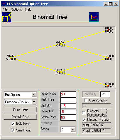
The above displays the values of the put option at each node, which is the value of your assumed position. At the initial node, the put is worth 9.68. The put value after an up-tick is 4.47 and after a down-tick is 20.24.

Our objective is to hedge the put option's price risk using the underlying stock. First, we will define a number referred to as Delta, which is useful when hedging option risk. Delta is a number that measures the change in the value of the option when the stock price changes. Denote it by the Greek letter , so that

Therefore, DS = DP, or DP - DS = 0, so if we hold - stocks, then the change in the put value will be mirrored by the change in the value of the - stocks.

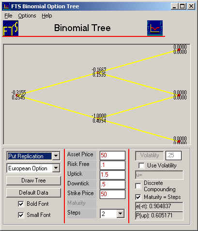
By selecting either the put or call replication from the drop down, the Binomial Tree Module will display the delta of the selected option at each node. For the current example put replication results in the following tree:

Creating a Riskless Position

At the initial node, is -0.3155. This means that to replicate a long (i.e., +1) put option we should sell 0.3155 stocks and lend the proceeds to the money market. But recall our goal is to create a riskless position when we already own one put option.

How do we do this?

The answer to is to replicate a short (i.e., -1 put option) position

To do this requires that we change the signs in a long synthetic put option position. That is, from a trading perspective we should borrow from risk free money market and buy 0.3155 stocks to replicate the short put option.

If we do this we can create a position that is completely riskless. That is, we are long one put option and simultaneously short one synthetic put option. The net effect eliminates all underlying asset price risk from the position. You can check, at the end of the first period, that your portfolio is worth $10.69 whether the stock ticks up or down. In other words, you have created synthetically a risk free bond.

Let us calculate the portfolio values to verify these numbers. In these calculations, we will assume that you started with one put option and no cash, so that if you buy stocks, you have to borrow money at the risk free interest rate (which is 10% or 0.10). This actually does not make any difference because you can assume you have some initial amount of cash, and conduct similar calculations.

Calculation at initial node: You started with one put option worth $9.92, and bought 0.3155 stocks. The stock price at the initial node is 50, so you had to borrow 0.3155 x 50 = 15.775. Your portfolio value is:

	Quantity	Value
Put Option	1	9.68
Stock	0.31552	15.776
Cash	-15.776	-15.776
	Total	9.68

Notice that the value of your stocks cancel the borrowings, so that your portfolio value equals the value of the put option you started with.

Suppose there is a down-tick in period 1: At this node, the stock price is 25 and the put is worth $20.24. Since the risk-free interest rate is 10%, you have to pay interest on the money you borrowed, so the net position is:

	Quantity	Value
Put Option	1	20.24
Stock	0.31552	7.888
Cash	-15.776	-17.4352
	Total	10.69

Suppose there is an up-tick in period 1: At this node, the stock price is 75 and the put is worth $4.47. Since the risk-free interest rate is 10%, you have to pay interest on the money you borrowed, so the net position is:

	Quantity	Value
Put Option	1	4.47
Stock	0.31552	23.664
Cash	-15.776	-17.4352
	Total	10.69

Calculation at node after initial down-tick

Now, the binomial tree for put replication indicates that delta is -1:

Since the delta is -1, you need to hold one stock when you leave this node. Since you have 0.31552 stocks, this means that you have to buy (1-.31552)=0.68448 more stocks. The stock price is 25, so you have to borrow an additional (0.68448*25)=17.112. Let us see what happens when you do buy the additional stocks. Note that your borrowings are now $34.5472 (= 17.4352 + 17.112).

If there is a subsequent down-tick (so there was a down-tick followed by a down-tick), you position will be:

	Quantity	Value
Put Option	1	37.50
Stock	1	12.50
Cash	-34.5472	-38.18
	Total	11.82

If there is a subsequent up-tick (so there was a down-tick followed by an up-tick):

	Quantity	Value
Put Option	1	12.50
Stock	1	37.50
Cash	-34.5472	-38.18
	Total	11.82

This confirms that your portfolio will be worth $11.82 along this path if you follow the trading strategy.

Now, let us complete the calculation for the case where there was an initial up-tick.

Calculation at node after initial up-tick

Now, the Binomial Tree for put replication tells you that the delta is -0.1667:

Since the delta is -0.1667, you need to reduce your stock holdings. You started with 0.3155, so you have to sell 0.1488 stocks. The stock price is 75, so you get $11.1637 from selling the stock. Your borrowings are therefore reduced to $6.2714, so in the next period, you will repay 6.2714 x exp(0.1) = 6.931. Let us see what happens.

If there is a subsequent down-tick (so there was an up-tick followed by a down-tick):

	Quantity	Value
Put Option	1	12.50
Stock	0.1667	6.25125
Cash	-6.2714	-6.931
	Total	11.82

If there is a subsequent up-tick (so there was an up-tick followed by an up-tick):

	Quantity	Value
Put Option	1	0
Stock	0.1667	18.75125
Cash	-6.2714	-6.931
	Total	11.82