hat is interesting about the two-period binomial model is that it allows determination of the option price by forming a riskless hedged portfolio from two securities, even though we have more than two terminal stock prices (Suu, Sud, Sdu, Sdd) and therefore more than two distinct call option values.

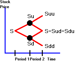
Figure 4.1

Binomial Tree for Stock Prices

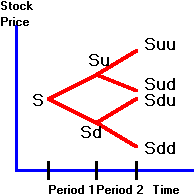
In Figure 4.1, the underlying asset value is path-dependent whenever Sud is not equal to Sdu.   Although the same principles apply to path-dependent and path-independent options, it is simpler to value path-independent options.  We therefore focus on them in this section.  If we assume that ud = 1, in which case Sud = Sdu = S, then multiple paths lead to the middle terminal node.   

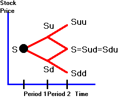
Figure 4.2

Binomial Tree:  Path Independent

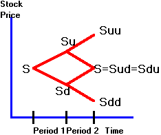
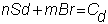
Then, after two periods, a call option with Sd < S < X < Su has payoffs:

Suu - X, S - X, and 0.

Now suppose you want to  form a synthetic call option from a portfolio of n stocks and m bonds.  How would you do this?  Observe that there are three possible end-of-period values to be replicated, but only two securities to work with.  The equations you have to solve are:

nSuu + m Br = Suu - X

nS + m Br = S - X

nSdd + m Br = 0

We have three equations and only two unknowns.  You know that one way of solving this is to create a portfolio of three securities but you also know that you can solve for the call price from a replicating portfolio of only two securities (the stock and the bond).

What is going on?

The answer lies in the ability to rebalance your position.  You do not have to hold your portfolio for two periods, but instead can re-trade at the end of the period.

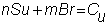
You may have observed in the two-period problem for a European call option, in Chapter 3, that the hedge ratio at each node is different.  In particular, the three hedge ratios are:

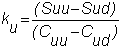
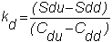
Thus, if you  create the riskless hedge portfolio at the beginning of the first period, you would have to adjust your position at the beginning of the second period to ensure that you have the appropriate hedge ratio.

You can apply this important principle by working with two of Option Tutor's  interactive subjects, Binomial Replication and Binomial Delta Hedging.  The software allows you to choose at each node the trade that should be executed either to maintain a riskless portfolio or to create a synthetic option.  You will see that the number of stocks required to maintain a riskless position changes at each node.  You can solve for such a position using the Binomial Delta subject in Option Tutor.

For now, let us work backward through the tree to try and create a synthetic option.

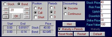
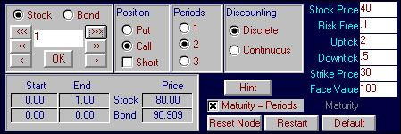
Online click on the Subject menu item and choose Binomial Replication.  Change the default values to stock price = $40, uptick = 2, riskfree = 0.10 (discrete compounding), strike price = 30.  Similarly select to display the call option with a two-period life.  Your screen should appear as follows:

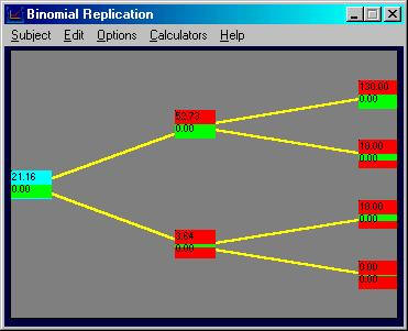
Click on the uptick node (currently labeled 52.73 and 0.00).  By choosing to go long 1 stock observe that the difference between the call option payoff, and the portfolio that has bought 1 stock (at $40), is $30.  You can see this as follows:

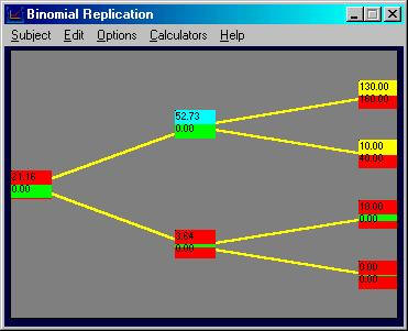
As a result, by introducing some riskfree bonds result in a synthetic call option being created.  In particular consider shorting (i.e., borrowing) 0.3 riskfree bonds with a terminal face value equal to $100.  This reduces the terminal node payoffs by $30 which results in a synthetic call option being constructed at the first uptick node.

Similarly we can construct a synthetic call option if we find that a downtick is realized resulting arriving at the node labeled 3.64.  Here the stock and bond position is 0.3333 stocks and -0.0333 bonds.  Note:  to control the 0.01 digit you can click on the button with a single >.  However, to control the 0.001 and 0.0001 digits to get to four decimal place accuracy, you need to type into the box 0.001 and click OK several times, and similarly for 0.0001.  If you want to subtract type in –0.0001 and click OK repeatedly.  After a little trial and error you will quickly control finer decimal places.

  That is, we are able to replicate the four terminal payoffs by using two stock/bond positions which are contingent upon which node is reached.

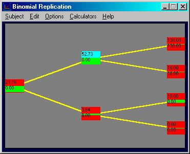
Finally, at the beginning node we can construct the synthetic call option by first clicking on this node and then by acquiring 0.81817 stocks (using the same trick as described above to control higher decimal places by typing in 0.00001 and clicking OK 7 times to add 0.00007) and selling 0.14 bonds as follows:

That is, at every possible node that you can reach there exists a position that can be constructed from stocks and bonds using the prevailing market prices that exactly mimics the call option.

This argument is presented for the general case as follows:

Consider the two nodes depicted as black dots in Figure 4.3.

Figure 4.3

Binomial Tree for Stock Values

To find the appropriate number of stocks and bonds to create a synthetic option, let n be the number of shares and m be the number of risk-free bonds. 

Then nu , nd , mu , md   are node-specific and must solve:

nu Suu + mu  Br  = Suu - X

nu S + mu  Br  = S - X

nd S + md  Br  = S - X

nd Sdd + md  Br  = 0.

We now have four equations and four unknowns.  From this set of equations, you can determine the synthetic form of Cu and Cd, as we did before.

Finally, step back to time 0, the first node.  Now there is only one node left (depicted by the black dot in Figure 4.4).

Figure 4.4

Initial Node Reached

Again, we need to find n and m to solve

where Cu and Cd are as obtained above. Once you solve these equations for n and m, you will know the price of the call option.

The important principle here is that the ability to trade at each node has the same effect as increasing the number of markets that are open.

Formally, trading increases the set of possible payoffs that we can achieve without having to open up additional markets.  Therefore, there is an interesting trade-off when hedging some risk.  The trade-off is between creating more complex portfolios as opposed to more frequent retrading of a smaller number of securities.

Rebalancing is the essence of Delta Hedging, our next topic.