n this topic, we show that you can use the one-period binomial model to value an option by creating a riskless portfolio using the stock and an option.  Here, riskless means that the portfolio has a known value at the end of the period, no matter what happens to the stock price. 

If the portfolio is riskless, then we know its current value; it is simply the future value discounted by the risk-free interest rate.  Then, since we know the portfolio value and the stock price, we can determine the option price.

Why are we doing this?  The answer comes from the general principle of valuation, which says that the value of an asset is the present discounted value of all future cash flows from the asset.  To value an option, we then need to determine two things: the future cash flows and the discount rate. 

For a European option, the future cash flows are easy; for example, for a call option, the cash flow is 0 if the future stock price is less than the strike price, and equals the future stock price minus the strike price otherwise.

What about the discount rate?  Here lies the problem.  We cannot use the risk-free interest rate, since the future cash flows are not risk-free; they depend on the unknown future stock price. If people are risk-averse, then they will hold risky securities only if they can get a return greater than the risk-free interest rate.  In fact, much of the problem in valuing risky securities is determining the appropriate discount rate, as in the capital asset pricing model. The fundamental riskless hedge argument solves the problem of determining the discount rate, since we know how to discount the riskless portfolio.

An example shows you how to create a riskless portfolio.  You can work through the example in this topic both numerically and graphically by using the Binomial Delta Hedging subject in Option Tutor.

Let S denote the current stock price and assume that at the end of one period the stock value is either 10 or 40.  We will study European put and call options with a strike price, X, of 20 when the risk-free interest rate is zero.

The future values of the stock and the options are depicted in the "tree" in Figure 2.1,

Figure 2.1

One-Period Binomial Tree

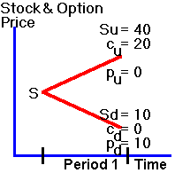
where, given an uptick, u, Su is the realized stock price, Cu is the realized call option value, and Pu   is the realized put option value.  You know, for instance, that Pu  is zero since the put option is worthless when S = 40 > X = 20.

Now suppose you form a portfolio:

Buy 2 stocks;

Sell 3 call options

Consider what happens at the end of the period if a downtick occurs.  Since the stock is worth 10, the call option finishes out-of-the-money and the trader you sold the call option to would not exercise it.  The final payoff from your portfolio is 20, which is the value of the two stocks.

Suppose an uptick occurs.  Each stock is worth 40, but the calls would now be exercised against you.  You would be required to give three stocks to the person who bought the options, and you would receive 20 for each stock.  Therefore, your final position would be:

+ 80 from the stock you hold;

+ 60 from the three options being exercised;

- 120 to buy the three stocks to give to the option exerciser;

which leaves you with 20.

Therefore, no matter what the state (or final value  of  the  stock), you will end up with 20 at the end of the period as indicated in Figure 2.2.

Figure 2.2

A Riskless Portfolio

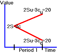
You now have a riskless portfolio.  The present value of this portfolio is 20 since we have assumed that the risk-free interest rate is zero.

This means that the portfolio that is long 2 stocks and short 3 call options must trade for a price equal to 20.  If not, there is an arbitrage opportunity.  To see this, suppose that you could sell such a portfolio for more than 20.  That is, 2S - 3C > 20, where S is the stock price and C is the call price.  Then, you can profit from selling this portfolio.  You receive more than 20 from the sale, but lose at most 20 at the end of the period, which ensures you of a profit.  Similarly, if you could buy this portfolio for less than 20, 2S - 3C < 20, then you can profit from buying it.

Each of these situations presents an arbitrage opportunity (i.e., the ability to make a sure return for zero wealth).  The only price at which arbitrage is not possible is if you can buy or sell this portfolio at 20, (2S - 3C = 20).

Since 2S - 3C = 20, we know that C = (2S - 20)/3, so if you know the price of the underlying stock, you know the value of the call option.

Puts can be priced in the same manner (by considering portfolios in which you buy stocks and buy puts).  You may want to verify that a portfolio consisting of one stock and three puts is worth 40 at expiration.   Since the portfolio costs S + 3P, we get S + 3P = 40, so P = (40 - S)/3 is the put price.

Positive Interest Rate

Our analysis so far assumes that the risk-free interest rate is zero.  Suppose instead the interest rate is some positive amount.  This assumption changes the analysis a little.  No longer is 20 an arbitrage-free price, because now there exists a better opportunity.

To see why, suppose at the beginning of the period you could sell 2S - 3C at 20.  You can now profit from selling this portfolio and investing the proceeds at the risk-free interest rate.  Let r = 1 + the risk-free interest rate.  At the end of the period you will receive 20r >20, and pay out 20. 

To eliminate this arbitrage opportunity, it must be the case that in the presence of a positive risk-free rate of interest 2S - 3C = 20/r.  Therefore the arbitrage-free option prices are obtained as before with this adjustment, C = (2S - 20/r)/3 and P = (40/r - S)/3.

The Binomial Delta Hedging subject in Option Tutor lets you rework this example for different interest rates. 

Summary

We have shown how to value an option by constructing a riskless portfolio.  We then use the fact that we know how to discount a riskless portfolio to obtain the value of the option.

A second approach to valuing options is to form a synthetic option exampleSOE_BIN  from the underlying asset and a bond.  An example of this approach is presented in the next topic.