 office (412)
9679367
office (412)
9679367D.5 Distribution
of Stock Prices
In
the geometric Brownian motion model of stock prices, the important assumptions
made on the random variable, z, are:
1.
The change in z is the product of a standard normal random variable (i.e., with
mean zero and standard deviation 1) and the square root of the interval of time. This implies that the variance
of stock prices increases linearly with time.
2.
For any two (non-overlapping and small) intervals of time, the change in z
is independent. This is consistent
with the (weak form of the) efficient markets hypothesis.
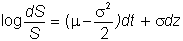
In
topic D.6, Derivation of Stock Price Distribution, we show that the log of the
instantaneous stock return follows the diffusion process below:
Assumptions
1 and 2, together with the equation describing the log of the instantaneous
stock return, give us a nice distribution for the stock price.
They imply that the random variable log(ST)-log(S),
which is the change in the stock price between now and period T,
is normally distributed with mean:

and
variance
Now,
if X is a random variable and log(X)
is normally distributed, then X itself
has a lognormal distribution.
In fact, this is the definition of the lognormal distribution.
As a result, at the end of any interval of time, the stock price is
lognormally distributed. If log(X)
is normally distributed with mean q and variance h2,
then the mean and variance of X are
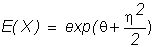
.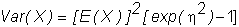
For
the case of the stock price, we have

and
.
Substituting
for these values, we find that the mean of ST
is:
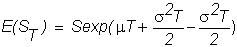
so
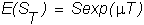
and
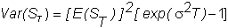
the variance of ST
is:
In
the next technical topic, Derivation of Stock
Price Distribution, we formally show that the log of the instantaneous stock
return follows the diffusion process shown.
This completes the characterization of the distributional properties for
stock prices which are implied from the geometric Brownian motion model.