D.2  Ito Processes

We start by defining (standard) Brownian motion.  Our treatment is informal, and if you are interested in pursuing the details and the derivations, we recommend you consult an advanced source such as Duffie (1988).

A stochastic process describes the evolution of a random variable through time.  Time can be modeled discretely or continuously.  Brownian motion is a special continuous time stochastic process that embodies the idea of "purely random" changes, where the randomness is captured by the normal distribution. 

Let x denote the value taken by the process.  For concreteness, think of x as the price of the stock.  At time t, x can take on many values, depending on the outcome of a random variable.  This randomness is modeled as follows. 

Let W be a set of states.  If state z occurs at time t, then the value of x is x(t,z).  The randomness is described by a probability distribution on  W. 

Brownian motion is a special process that satisfies these assumptions:

1.  D(s,t) = x(.,t) - x(.,s) is normally distributed for any t > s, with mean zero and variance (t - s) over the time interval (t - s).

2. If we take any n non-overlapping intervals of time, then D(s1,t1), D(s2,t2),...,D(sn,tn) are all independent.

The first property says that price changes are normally distributed while the second property says that all price changes are independent.  The first assumption also says that the variance increases linearly with time, and the expected price change is zero.

Brownian motion comes very close to how we expect returns to behave in an efficient market.  Market efficiency is the notion that the stock price embodies all available information, and therefore price changes are unpredictable.  If price changes are normally distributed, then Brownian motion provides a nice way to formalize this notion.

You may find a "discrete time" analogue useful.  Think of the change in z, Dz, in the period of time Dt, as being described by

where e is a normally distributed, random variable with mean zero and standard deviation 1, and changes in z over two non-overlapping intervals of time are independent.  Then,

 E(Dz) = DtE(e) = 0

and

var(Dz) = (Dt)var(e) = Dt. 

Brownian motion is the limit of this process when Dt goes to zero.

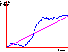
While Brownian motion may be a nice model of returns, it is not quite as nice a model of stock prices.  Figure D.1 is more what we want to capture.  

Figure D.1

Stock Price as a Function of Time

Here, price changes are random, but have a positive drift.  This type of behavior is captured by a diffusion process.  A diffusion process in its general form is written as

where z is Brownian motion and a is the drift term (which can depend on both x and t).  It controls the deterministic growth rate of the process.  b is called the volatility term (and can also depend on both x and t).  The volatility controls how much the process is affected by the random changes.

The most common model of stock prices imposes a special structure on the drift and volatility terms.  This is the model we have been using, and it is written as follows:

Here, the drift and the volatility do not depend on time, but do depend on the stock price.  If you divide both sides by S, you will get

The left-hand side is called the instantaneous return, and it is made up of two factors.  The first is mdt, which is the deterministic change in S.  The second is due to the change in z, multiplied by a positive number,  s. 

The number  m is called the drift rate of S and  s is called the volatility.

This is the equation that Black and Scholes use to model the behavior of a stock price.  It is often referred to as "geometric Brownian motion."  It says that S is expected to grow at rate m at an instant of time, and the instantaneous return, dS/S, is normally distributed.

You can see that if  s = 0, the stock has zero volatility, and then

which is the constant growth  process when there is no uncertainty.

The price of a derivative security, such as an option or a futures contract, is typically a function of time and the underlying stock price.  Generally, we can write this as a function f(x,t).  Of central importance is  Ito's Lemma (topic D.3), which allows the price dynamics for the derivative to be derived.  In addition, an application of this lemma allows both the Black-Scholes Partial Differential Equation (topic D.4) and the Distribution of Stock Prices ( topic D.6) to be derived.

previous topic

next topic

(C) Copyright 1999, OS Financial Trading System