The objectives for this section are:

i. To examine the scatter plot of returns over time,

ii. To test the null hypothesis that returns are normally distributed

iii. To examine the behavior of volatility over time.

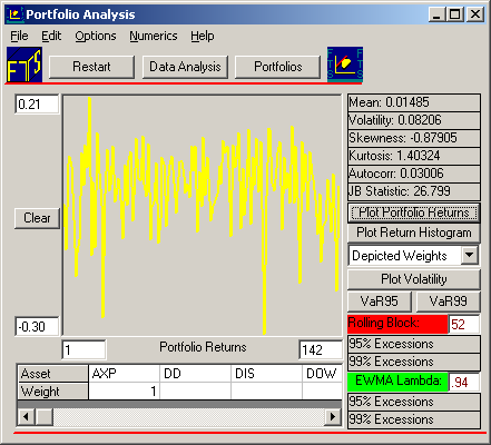
We start with looking at i. for American Express (AXP).

Select Depicted Weights (the default below the button Plot Return Histogram) and enter a 1 under AXP leaving all other stock weight fields blank (see above). Then first click on the Plot Portfolio Returns buttons. This plots the realized (in this case monthly) returns over time. We are interested in whether they appear to be randomly changing over time plus whether they exhibit any systematic characteristic such as clusters of more volatile (widely dispersed) over sub periods of time. A scatter plot of returns lets you become familiar with the data visually which is an important first step.

For example, if returns exhibit non random behavior over time then this is inconsistent with weak form of market efficiency. The indication of the extent to which it is serially correlated is provided by the Autocorrelation statistic. For the case of AXP this is low (0.030).

Similarly, if volatility of returns tend to cluster into high and low regimes over time this is also inconsistent with the weak form of market efficiency. For risk management purposes we are interested in the behavior of extreme negative returns which this module lets you analyze.

Our immediate goal, however, is to test whether observed returns come from the stationary and symmetrical Normal Distribution.